This vignette assumes that you have already been able to set up the connection to a Moodle Database and created a local cache (if chosen).
Data access functions
Learning analytics practitioners working with LMS data will often be interested in a sub-set of the available tables with relevant references added. These can be accessed through several mdl_* functions which will connect to the relevant table(s) and return a reference to the data. Currently the package supports curated access through the following functions:
For example:
my_grades <- mdl_grades()creates an R object named my_grades containing the dbplyr reference to the table in question.
Summary functions
The R generic summary function is implemented with sensible defaults so that:
summary(my_grades)
#> ----------
#> # of Grades:      1.4M
#> Missing:      945.2K
#> Courses:      2.8K
#> Users:        22.9K
#> Normalized Grades:
#> Median:       0.967
#> Mean:         0.859
#> SD:           0.336
provides useful information for the learning analytics practitioner.
Plot functions
Generic plot functions are also provided for all data-access objects:
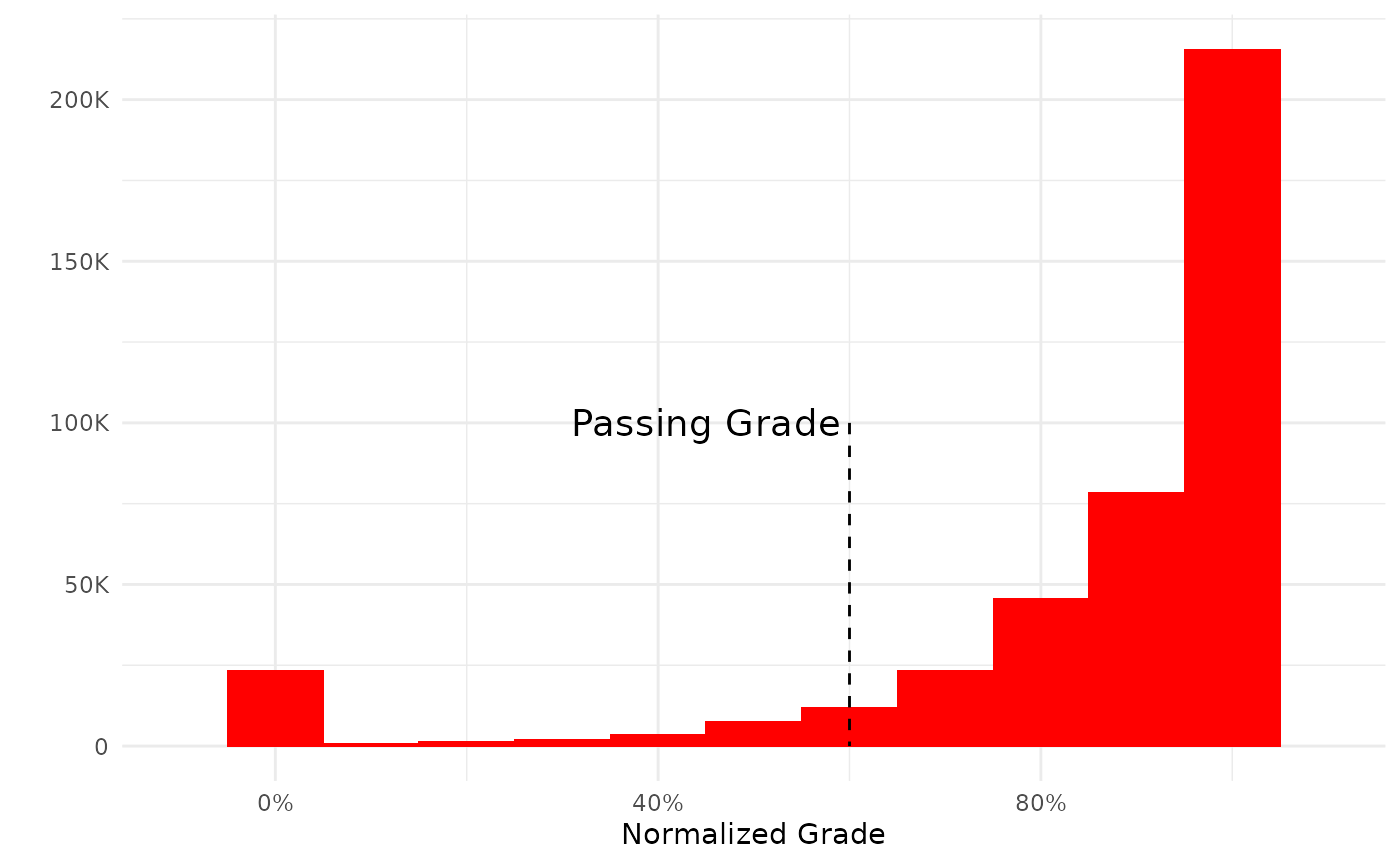
plot(my_grades)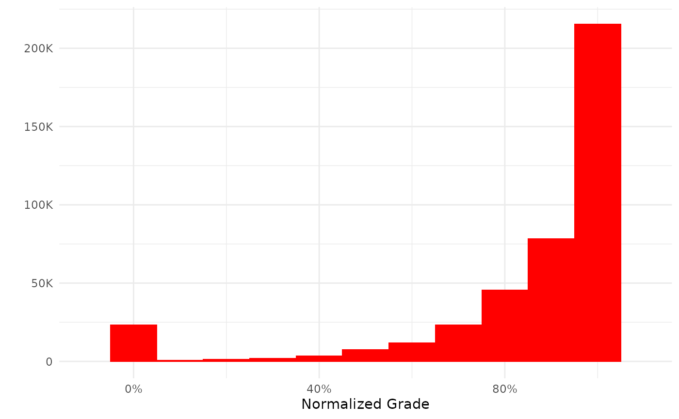
The plot functions return a ggplot by default. If you prefer base graphics you can call the function thus:
plot(my_grades, use_base_graphics = TRUE)
Additional columns
For convenience some additional columns have been added to the tables. These are all snake_case and are thus easy to spot:
Objects of class dbplyr
The return value from the data-access functions are also dbplyr tables so dbplyr verbs and operation work on them as well. For example:
my_grades %>%
  filter(courseid == 4957) %>%
  summary()
#> ----------
#> # of Grades:      99
#> Missing:      27
#> Courses:      1
#> Users:        11
#> Normalized Grades:
#> Median:       0.956
#> Mean:         0.950
#> SD:           0.043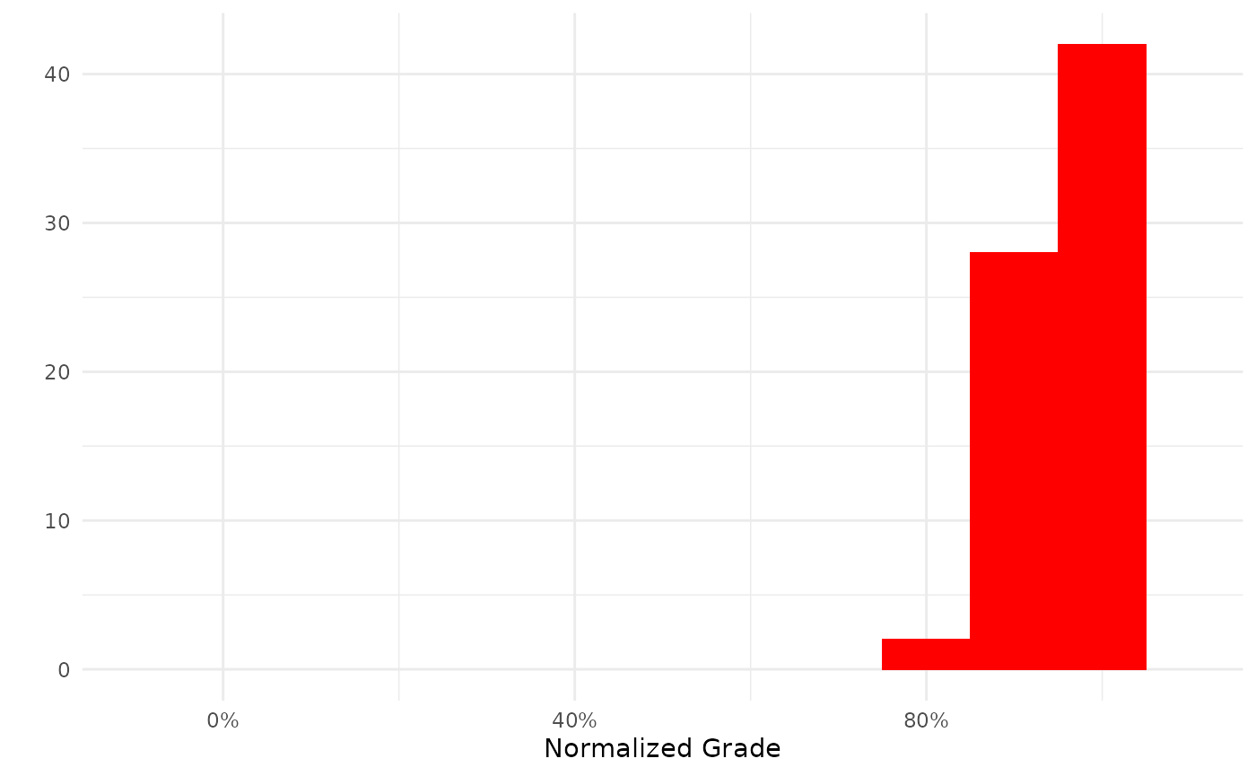
Using ggplot objects
Since the return value of a plot function is a ggplot object it is of course possible to add and/or manipulate the plot using the syntax from the ggplot2 package. For example by annotating the plot:
my_plot <- mdl_grades() %>%
  plot()
my_plot +
  annotate("text",.45,10^5, label="Passing Grade",cex=5)+
  annotate("segment",x=.6,y=10^5,xend=.6,yend=0, lty=2)