The algorithm is guaranteed to converge to an optimal policy for each possible state in \(S\). RL (and in this case we will use Q-learning) needs to be trained on a set of state-transition tuples formally defined in eq-tuples. \[
(s_i, a_i, r_{i+1}, s_{i+1})
\tag{2.1}\]
Reducing our Spaces
For our \(S\) as defined above the number of possible states is \(10^{60}\), which is a 1 followed by 60 zeros, i.e.:
      |\__/,|   (`\
    _.|o o  |_   ) )
---(((---(((---------
Wow, that's a huge number!
\(10^{60}\) = 1,000, 000, 000, 000, 000, 000, 000, 000, 000, 000, 000, 000, 000, 000, 000, 000, 000, 000, 000, 000.
The action space \(A\) is slightly smaller since there are only four possibilities for each cell, so we have “only” \(4^{60}\) which is roughly equal to \(1.329\times10^{36}\).
Given the magnitude of these numbers it is clear that we cannot reasonably expect the algorithm to converge for several millennia with the computing power currently at our disposal. We therefore need to employ some strategies for reducing the spaces.
One Type at a Time
We can consider a one-type-at-a-time strategy. The heuristic implemented would then be to first look for moves involving candy, then move on to trees and so on. For example: staring with an initial board like this:
\[\begin{bmatrix} G & C & J & D & G & G & C & G & B & A \\ I & D & E & A & C & B & H & C & E & F \\ J & C & J & F & C & J & A & H & B & F \\ H & C & D & F & C & F & D & B & G & B \\ D & I & H & I & I & B & F & C & C & E \\ B & F & A & J & E & H & I & C & H & G \end{bmatrix}\]
And chose to consider the “A” cells we get:
\[\begin{bmatrix} 0 & 0 & 0 & 0 & 0 & 0 & 0 & 0 & 0 & 0 \\ 0 & 0 & 0 & 0 & 0 & 0 & 0 & 0 & 0 & 0 \\ 1 & 0 & 0 & 0 & 0 & 0 & 0 & 0 & 0 & 0 \\ 0 & 0 & 1 & 0 & 0 & 0 & 0 & 1 & 1 & 0 \\ 0 & 1 & 0 & 0 & 0 & 0 & 0 & 0 & 0 & 0 \\ 0 & 0 & 0 & 0 & 0 & 0 & 1 & 1 & 0 & 0 \end{bmatrix}\]
This reduces the problem to a binary one and we effectively reduce \(S\) to \(2^{60}\), which is merely 1.15 quintillions. While this represents a huge reduction, it is still far from being feasible. In addition this does not reduce our action space \(A\), as you still have four possible moves for each of the 60 cells.
Windowing
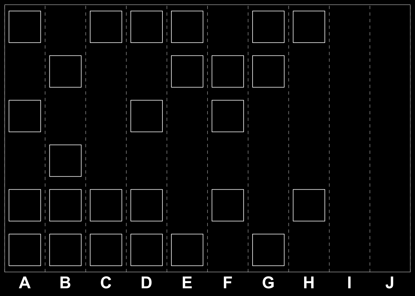
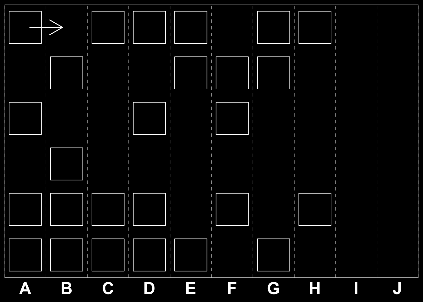
We can further reduce our problem space by applying a technique known as windowing. This implies dividing the grid into sub-grids and looking for playable moves within those reduced spaces. If we first consider the quest for a three-tile combinations, the windows in question would be a \(3\times2\) and a \(2\times3\) sub-matrix for perpendicular (\(\perp\))moves. For parallel (\(\parallel\)) moves, i.e. moves with the same row or column we would have to consider \(1\times4\) and \(4\times1\) respectively. Examples are shown below.
\[\begin{bmatrix} 1 & 1 & 0 \\ 0 & 1 & 1 \end{bmatrix}
%
\text{ or}
%
\begin{bmatrix} 1 & 0 \\ 1 & 1 \\ 0 & 1 \end{bmatrix}
%
\text{ for }\perp\text{moves,}\]
and
\[\begin{bmatrix} 1 & 1 & 0 & 1 \end{bmatrix}
%
\text{ or}
%
\begin{bmatrix} 1 \\ 1 \\ 0 \\ 1 \end{bmatrix}
%
\text{ for }\parallel \text{ moves.}\]
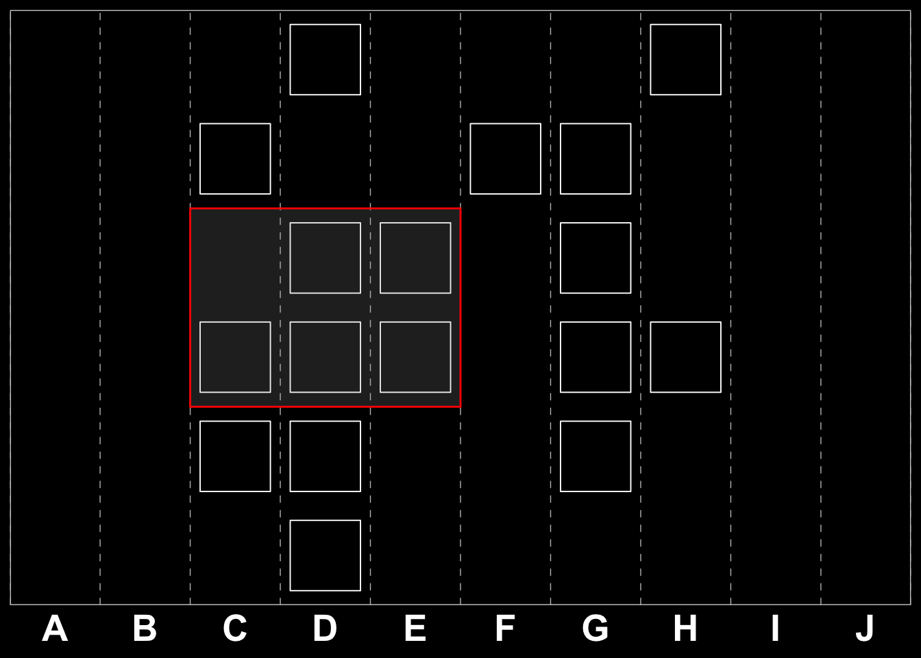
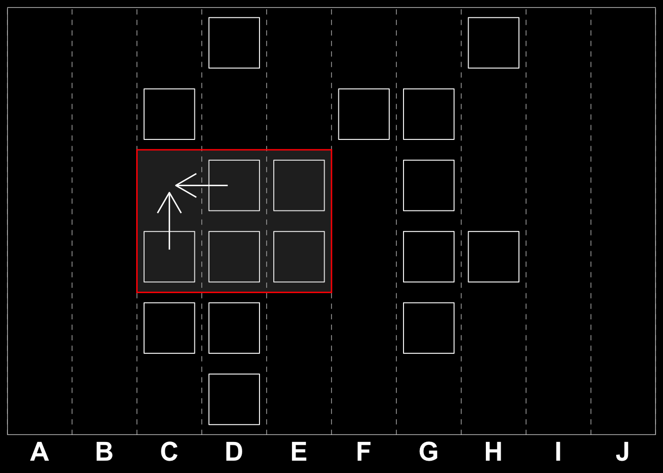
Is it easy to see that the \(3\times2\) matrix above is a transposition of the \(2\times3\) one, and therefore it does not matter whether a move if horizontal or vertical the problem is similar in nature for all perpendicular moves. The same is true for the \(4\times1\) and \(1\times4\) matrices, i.e. where there is a winning parallel move. Matrix eq-example-windows illustrates two windows on our original board and Matrix eq-example-windows-binary shows the same in our binary space (combining the two reduction strategies).
\[
\begin{bmatrix} G & \color{red}{\textbf{C}} & \color{red}{\textbf{J}} & \color{red}{\textbf{D}} & \color{red}{\textbf{G}} & G & C & G & B & A \\ I & D & E & A & C & B & H & C & E & F \\ J & C & J & F & C & J & \color{red}{\textbf{A}} & \color{red}{\textbf{H}} & B & F \\ H & C & D & F & C & F & \color{red}{\textbf{D}} & \color{red}{\textbf{B}} & G & B \\ D & I & H & I & I & B & \color{red}{\textbf{F}} & \color{red}{\textbf{C}} & C & E \\ B & F & A & J & E & H & I & C & H & G \end{bmatrix}
\tag{2.2}\]
\[
\begin{bmatrix}
0 & \color{red}{\textbf{1}} & \color{red}{\textbf{0}} & \color{red}{\textbf{0}} & \color{red}{\textbf{0}} & 0 & 1 & 0 & 0 & 0 \\
0 & 0 & 0 & 0 & 1 & 0 & 0 & 1 & 0 & 0 \\
0 & 1 & 0 & 0 & 1 & 0 & \color{red}{\textbf{0}} & \color{red}{\textbf{0}} & 0 & 0 \\
0 & 1 & 0 & 0 & 1 & 0 & \color{red}{\textbf{0}} & \color{red}{\textbf{0}} & 0 & 0 \\
0 & 0 & 0 & 0 & 0 & 0 & \color{red}{\textbf{0}} & \color{red}{\textbf{1}} & 1 & 0 \\
0 & 0 & 0 & 0 & 0 & 0 & 0 & 1 & 0 & 0
\end{bmatrix}
\tag{2.3}\]
The Reduced Action Spaces
If we employ the windowed approach suggested above, our action space, \(A\) shrinks significantly. We will in fact have two different \(S\) and \(A\) depending on whether we are considering parallel or perpendicular moves.
For a parallel window, we can generalize to the horizontal variant (since the horizontal one is a simple transposition thereof) and we then get only a few relevant combinations. Since any four element set which already has three in a row is will not occur, we are left with: {0000,0001,0010,0011,0100,0101,0110,1000,1001,1011, 1101} for a total of 11 cases out of which only two have a winning move ({1011, 1101}). This reduces \(A_{\parallel}\) for \(S_{\parallel}\) to three moves: pass (P), flip first (F) or flip last (L). formalized in Equation eq-action-space-parallel.
\[
A_{\parallel} = \{P,F,L\}
\tag{2.4}\]
For the perpendicular case we 62 combinations, these are illustrated in Equation eq-perpendicular-combinations.
\[
S_{\perp} = \Biggl\{ \left[{000\atop{000}}\right],
\left[{000\atop{001}}\right],
\left[{000\atop{010}}\right] ...
\left[{001\atop{001}}\right],
\left[{001\atop{010}}\right]...
\left[{110\atop{011}}\right]
\Biggr\}
\tag{2.5}\]
The action space is limited to flipping one out of three positions, First, Middle, Last, or Passing. Illustrated in Equation eq-action-space-perpendicular.
\[
A_{\perp}=\{F,M,L,P\}
\tag{2.6}\]